Navier-Stokes Equations
The Navier–Stokes equations mathematically express conservation of momentum and conservation of mass for Newtonian fluids. A laminar flow example: The higher-order term, namely the shear stress divergence ∇ · τ, has simply reduced to the vector Laplacian term μ∇2u. This Laplacian term can be interpreted as the difference between the velocity at a point and the mean velocity in a small surrounding volume. This implies that – for a Newtonian fluid – viscosity operates as a diffusion of momentum, in much the same way as the heat conduction. In fact neglecting the convection term, incompressible Navier–Stokes equations lead to a vector diffusion equation (namely Stokes equations), but in general the convection term is present, so incompressible Navier–Stokes equations belong to the class of convection–diffusion equations.
Incompressible Navier–Stokes equations (convective form):

Lagrangian and Eulerian approach
Lagrangian specification of the flow field is a way of looking at fluid motion where the observer follows an individual fluid parcel as it moves through space and time. Plotting the position of an individual parcel through time gives the pathline of the parcel. This can be visualized as sitting in a boat and drifting down a river.
The Eulerian specification of the flow field is a way of looking at fluid motion that focuses on specific locations in the space through which the fluid flows as time passes. This can be visualized by sitting on the bank of a river and watching the water pass the fixed location.
Material derivative
In continuum mechanics, the material derivative describes the time rate of change of some physical quantity (like heat or momentum) of a material element that is subjected to a space-and-time-dependent macroscopic velocity field. The material derivative can serve as a link between Eulerian and Lagrangian descriptions of continuum deformation.
For example, in fluid dynamics, the velocity field is the flow velocity, and the quantity of interest might be the temperature of the fluid. In which case, the material derivative then describes the temperature change of a certain fluid parcel with time, as it flows along its pathline (trajectory).
Suppose we have a flow field u, and we are also given a generic field with Eulerian specification F(x,t). Now one might ask about the total rate of change of F experienced by a specific flow parcel. This can be computed as
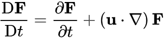
where ∇ denotes the nabla operator with respect to x, and the operator u⋅∇ is to be applied to each component of F. This tells us that the total rate of change of the function F as the fluid parcels moves through a flow field described by its Eulerian specification u is equal to the sum of the local rate of change and the convective rate of change of F.
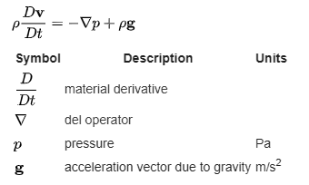
Incompressible Newtonian fluid
For the special (but very common) case of incompressible flow, the momentum equations simplify significantly. Using the following assumptions:
- Viscosity
 will now be a constant
- The second viscosity effect

- The simplified mass continuity equation

This gives incompressible Navier Stokes equations, describing incompressible Newtonian fluid:

Inviscid flow
Inviscid flow is the flow of an inviscid fluid, in which the viscosity of the fluid is equal to zero. Assuming inviscid flow allows the Euler equation to be applied to flows in which viscous forces are insignificant. Some examples include flow around an airplane wing, upstream flow around bridge supports in a river, and ocean currents. In a 1757 publication, Leonhard Euler described a set of equations governing inviscid flow:
No-slip and No-penetration boundary conditions
The no-slip condition for viscous fluids assumes that at a solid boundary, the fluid will have zero velocity relative to the boundary.
The fluid velocity at all fluid–solid boundaries is equal to that of the solid boundary. Conceptually, one can think of the outermost molecules of fluid as stuck to the surfaces past which it flows. Because the solution is prescribed at given locations, this is an example of a Dirichlet boundary condition.
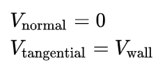
While the no-slip condition is used almost universally in modeling of viscous flows, it is sometimes neglected in favor of the ‘no-penetration condition’ (free-slip, where the fluid velocity normal to the wall is set to the wall velocity in this direction, but the fluid velocity parallel to the wall is unrestricted) in elementary analyses of inviscid flow, where the effect of boundary layers is neglected.
Ordinary Differential Equations (ODE) and Partial Differential Equations (PDE)
An ordinary differential equation (ODE) is a differential equation containing one or more functions of one independent variable and the derivatives of those functions. The term ordinary is used in contrast with the term partial differential equation which may be with respect to more than one independent variable.
Partial differential equation (PDE) is an equation which imposes relations between the various partial derivatives of a multivariable function. The function is often thought of as an “unknown” to be solved for, similarly to how x is thought of as an unknown number, to be solved for, in an algebraic equation like x2 − 3x + 2 = 0. However, it is usually impossible to write down explicit formulas for solutions of partial differential equations. There is, correspondingly, a vast amount of modern mathematical and scientific research on methods to numerically approximate solutions of certain partial differential equations using computers. Partial differential equations also occupy a large sector of pure mathematical research, in which the usual questions are, broadly speaking, on the identification of general qualitative features of solutions of various partial differential equations.
Matrix multiplication
In mathematics, particularly in linear algebra, matrix multiplication is a binary operation that produces a matrix from two matrices. For matrix multiplication, the number of columns in the first matrix must be equal to the number of rows in the second matrix. The resulting matrix, known as the matrix product, has the number of rows of the first and the number of columns of the second matrix.
If A is an m × n matrix and B is an n × p matrix, the matrix product C = AB (denoted without multiplication signs or dots) is defined to be the m × p matrix.


